Crime analysis examples

All the files from https://data.police.uk/data/ has been downloaded as CSV files and processed to form a single table in a postgis (spatial) databases. The individual files consist of around 50 csvs for each month of the year from October 2018 to September 2021 (i.e. over 1500 files). The data can be grouped in many different ways and queried much more rapidly than through using the online api.

dbListFields(con,"crimes2")

## [1] "reported_by"           "lsoa_code"             "crime_type"           
## [4] "last_outcome_category" "date"                  "geometry"

dbGetQuery(con,"select distinct crime_type from crimes2") %>% aqm::dt()

Show entries

Search:

	crime_type

1	Vehicle crime
2	Other crime
3	Violence and sexual offences
4	Criminal damage and arson
5	Possession of weapons
6	Robbery
7	Drugs
8	Burglary
9	Public order
10	Theft from the person

Showing 1 to 10 of 14 entries

Previous1 2Next

Find all the violent crimes that were recorded in April 2021. Filter the results by outcome.

query<-"select * from crimes2 where crime_type like '%Viol%' and date between '2021-04-01' and '2021-05-01'"
dd<-st_read(con, query=query)
dd %>% filter(str_detect(last_outcome_category, "Offender") | str_detect(last_outcome_category, "court") ) -> dof

dd %>% st_drop_geometry() %>%  group_by(last_outcome_category) %>% summarise(n=n()) %>% arrange(n) %>% mutate(last_outcome_category = factor(last_outcome_category, last_outcome_category)) -> df
ggplot(df, aes(x=last_outcome_category,y=n)) +geom_col() + coord_flip()

dof %>% st_drop_geometry() %>%  group_by(last_outcome_category) %>% summarise(n=n()) %>% arrange(n) %>% mutate(last_outcome_category = factor(last_outcome_category, last_outcome_category)) -> df
ggplot(df, aes(x=last_outcome_category,y=n)) +geom_col() + coord_flip()

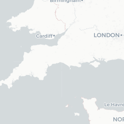
dof %>% mapview(zcol='last_outcome_category', burst=TRUE, legend=FALSE) ->mp
  mp@map %>% addSearchOSM(options = searchOptions(autoCollapse = TRUE, minLength = 2)) %>%
    addFullscreenControl()

Find all the violent crimes that were recorded by Dorset police. Filter the results by outcome.

query<-"select * from crimes2 where crime_type like '%Viol%' and reported_by like '%Dorset%'"
dd<-st_read(con, query=query)
dd %>% filter(str_detect(last_outcome_category, "Offender") | str_detect(last_outcome_category, "court") ) -> dof

dd %>% st_drop_geometry() %>% group_by(date) %>% summarise(n=n()) ->dts
library(xts)
library(dygraphs)
dygraph(xts(dts$n,dts$date))

dd %>% st_drop_geometry() %>%  group_by(last_outcome_category) %>% summarise(n=n()) %>% arrange(n) %>% mutate(last_outcome_category = factor(last_outcome_category, last_outcome_category)) -> df
ggplot(df, aes(x=last_outcome_category,y=n)) +geom_col() + coord_flip()

dof %>% st_drop_geometry() %>%  group_by(last_outcome_category) %>% summarise(n=n()) %>% arrange(n) %>% mutate(last_outcome_category = factor(last_outcome_category, last_outcome_category)) -> df
ggplot(df, aes(x=last_outcome_category,y=n)) +geom_col() + coord_flip()

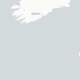
dof %>% mapview(zcol='last_outcome_category', burst=TRUE, legend=FALSE) ->mp
  mp@map %>% addSearchOSM(options = searchOptions(autoCollapse = TRUE, minLength = 2)) %>%
    addFullscreenControl()

Crime analysis examples

Using the postgis data base